4. The Discount Factor

Jun He June 02, 2026

中文English 一价定律Law of One Price 贴现因子Discount Factor 无套利No-Arbitrage 正贴现因子Positive SDF 分离超平面Separating Hyperplane

4. The Discount Factor

Note

本章导读本章（Cochrane 第 4 章）问一个更基本的问题：贴现因子 $m$ 从哪来？ 答案出人意料地廉价。仅凭价格与支付的两条性质，就能反推出 $m$ 的存在与正性，完全不必假设效用、完全市场或均衡。§4.1 一价定律 (law of one price) $\Rightarrow$ 存在一个支付空间内的贴现因子 $x^*$，并给出显式构造 $x^*=p'\mathbb E(xx')^{-1}x$；§4.2 无套利 (no-arbitrage) $\Rightarrow$ 存在严格为正的贴现因子 $m>0$（由分离超平面定理给出，但不唯一）；§4.3 $x^*$ 的另一种（均值-协方差）表达式，及其连续时间形式。

4. The Discount Factor

Note

Overview This chapter (Cochrane Ch 4) asks a more basic question: where does the discount factor $m$ come from? The answer is surprisingly cheap. From just two properties of prices and payoffs we can back out the existence and positivity of $m$ — with no assumption of utility, complete markets, or equilibrium. §4.1 the law of one price $\Rightarrow$ there exists a discount factor $x^*$ inside the payoff space, with the explicit construction $x^*=p'\mathbb E(xx')^{-1}x$; §4.2 no-arbitrage $\Rightarrow$ there exists a strictly positive discount factor $m>0$ (delivered by the separating hyperplane theorem, but not unique); §4.3 an alternative (mean-covariance) expression for $x^*$ and its continuous-time form.

4.1 一价定律与贴现因子的存在 / Law of One Price and the Existence of a Discount Factor

我们一直把 $p=\mathbb E(mx)$ 当作出发点。本节反过来：把价格与支付当作原始对象，问什么条件下能找到一个 $m$ 使 $p=\mathbb E(mx)$ 成立。设支付空间为 $X$（可交易的支付集合），定价函数 $p(x)$ 把每个支付映到今天的价格。我们只要求 $p(\cdot)$ 满足两条性质：

4.1 Law of One Price and the Existence of a Discount Factor

We have been treating $p=\mathbb E(mx)$ as a starting point. This section turns it around: take prices and payoffs as the primitive objects, and ask under what conditions we can find an $m$ such that $p=\mathbb E(mx)$ holds. Let $X$ be the payoff space (the set of tradeable payoffs), and let the pricing function $p(x)$ map each payoff to its price today. We require only two properties of $p(\cdot)$:

A1（组合构造 / portfolio formation）：$x_1,x_2\in X\Rightarrow ax_1+bx_2\in X$（支付空间对线性组合封闭）。
A2（一价定律 / law of one price）：定价是线性的，

A1 (portfolio formation): $x_1,x_2\in X\Rightarrow ax_1+bx_2\in X$ (the payoff space is closed under linear combinations).
A2 (law of one price): pricing is linear,

$$p(ax_1+bx_2)=a\,p(x_1)+b\,p(x_2).$$

A2 即"一价定律"：同一支付无论由哪些证券组合而成，价格都相同——否则可低买高卖。注意 A1、A2 都很弱：不需要完全市场（$X$ 可以是 $\mathbb R^S$ 的真子空间），不需要无套利，更不需要效用或均衡。仅此两条就足以得到一个贴现因子：

A2 is the "law of one price": the same payoff has the same price no matter which securities are combined to form it — otherwise one could buy low and sell high. Note A1 and A2 are both weak: no complete markets (X may be a proper subspace of $\mathbb R^S$), no no-arbitrage, and certainly no utility or equilibrium. These two alone suffice to deliver a discount factor:

Important

贴现因子存在定理 / Existence theorem 在 A1、A2 下，存在唯一一个支付 $x^*\in X$，使得对每个 $x\in X$ 都有 $p(x)=\mathbb E(x^*x)$。这个 $x^*$ 就是一个（在支付空间内的）贴现因子。Given A1 and A2, there exists a unique payoff $x^*\in X$ such that $p(x)=\mathbb E(x^*x)$ for every $x\in X$. This $x^*$ is a discount factor (one that lives inside the payoff space).

证明一（几何 / 构造）。 关键的数学事实是：任何线性函数都可表示为内积。在支付空间 $X$ 上以 $\mathbb E(xy)$ 为内积，定价 $p(\cdot)$ 是 $X$ 上的线性函数，故存在某个 $x^*\in X$ 使 $p(x)=\mathbb E(x^*x)$。几何上：价格为 1 的支付构成一张超平面（"$\text{Price}=1$"），价格为 0 的支付（超额收益）构成过原点、与之平行的超平面。沿这些平面的法线方向取一个向量，调到合适长度，使其在 $\text{Price}=1$ 平面上的支付的内积恰为 1，这个向量就是 $x^*$。无穷维情形由 Riesz 表示定理 保证（Hansen and Richard 1987）。

Proof 1 (geometric / constructive). The key mathematical fact is that any linear function can be represented as an inner product. Equip the payoff space $X$ with the inner product $\mathbb E(xy)$; pricing $p(\cdot)$ is a linear function on $X$, so there is some $x^*\in X$ with $p(x)=\mathbb E(x^*x)$. Geometrically: the payoffs with price 1 form a hyperplane ("$\text{Price}=1$"), and the price-0 payoffs (excess returns) form a parallel hyperplane through the origin. Take a vector along the normal to these planes and scale it so that its inner product with any price-1 payoff equals 1 — that vector is $x^*$. The infinite-dimensional case is guaranteed by the Riesz representation theorem (Hansen and Richard 1987).

下图画出了这一几何：$\text{Price}=0$、$\text{Price}=1$、$\text{Price}=2$ 是一族平行的等价格线，$x^*$ 沿它们的公共法线方向，长度恰好使其落在 $\text{Price}=1$ 线上。

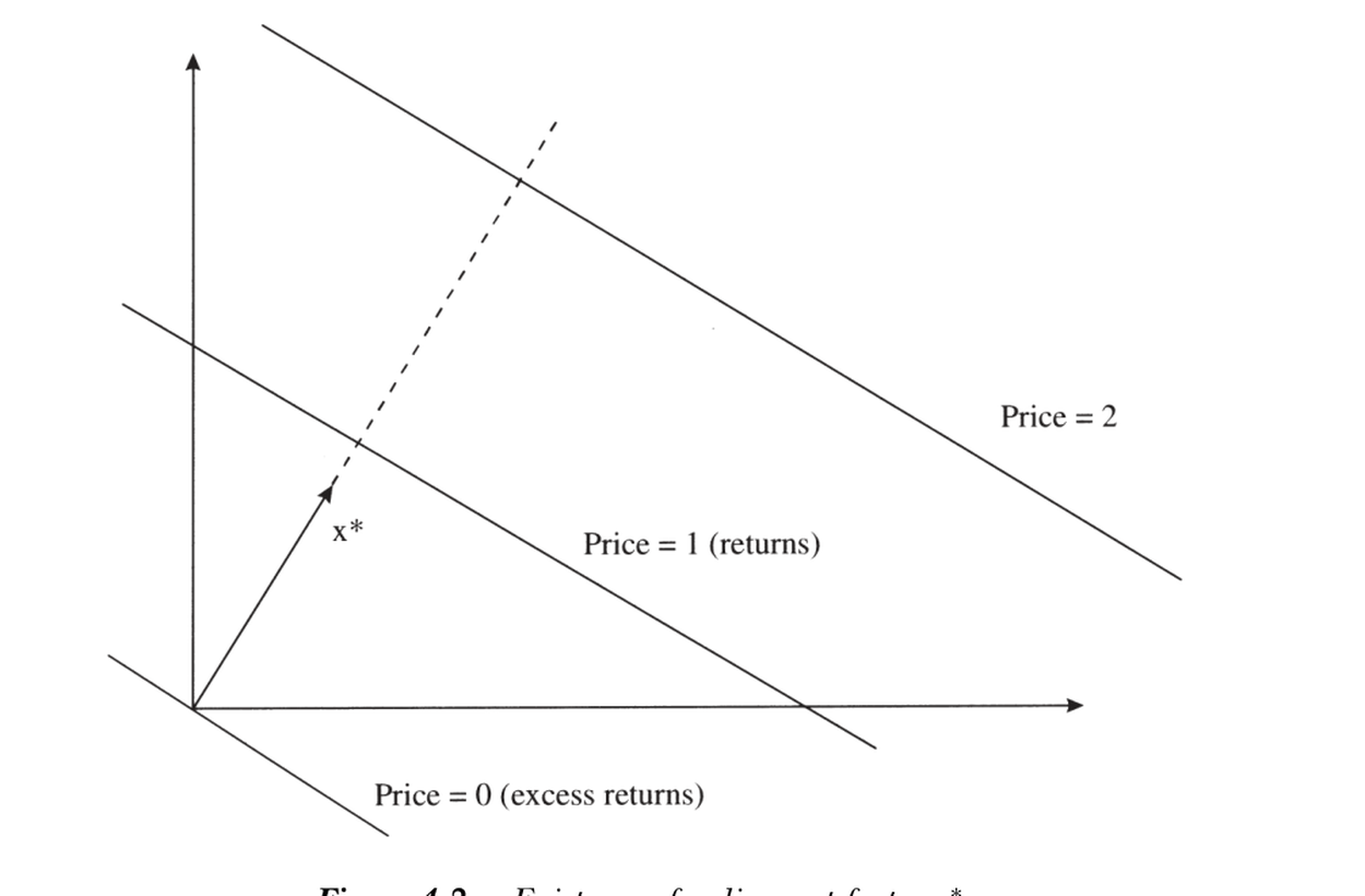
图 4.2　贴现因子 $x^*$ 的存在性。等价格线相互平行，$x^*$ 沿其公共法线，长度使其位于 $\text{Price}=1$ 线上。

Figure 4.2　Existence of a discount factor $x^*$. The constant-price lines are parallel; $x^*$ lies along their common normal, scaled to sit on the $\text{Price}=1$ line.

证明二（代数 / 构造）。 当支付空间由 $N$ 个基础支付张成时（例如 $N$ 只股票），可显式构造。把基础支付排成向量 $x=[x_1\;x_2\;\cdots\;x_N]'$，对应价格 $p$，支付空间 $X=\{c'x\}$。我们要找形如 $x^*=c'x$ 的贴现因子，使它给基础资产定出正确价格：$p=\mathbb E(x^*x)=\mathbb E(xx'c)=\mathbb E(xx')c$。于是 $c=\mathbb E(xx')^{-1}p$（A2 保证 $\mathbb E(xx')$ 非奇异），代回得显式公式：

Proof 2 (algebraic / constructive). When the payoff space is generated by $N$ basis payoffs (e.g. $N$ stocks), we can construct $x^*$ explicitly. Stack the basis payoffs into a vector $x=[x_1\;x_2\;\cdots\;x_N]'$ with prices $p$, so $X=\{c'x\}$. We seek a discount factor of the form $x^*=c'x$ that prices the basis assets correctly: $p=\mathbb E(x^*x)=\mathbb E(xx'c)=\mathbb E(xx')c$. Hence $c=\mathbb E(xx')^{-1}p$ (A2 guarantees $\mathbb E(xx')$ is nonsingular), and substituting back gives the explicit formula:

$$x^*=p'\,\mathbb E(xx')^{-1}\,x.\tag{4.1}$$

这个公式在实证中非常有用：给定一组资产的价格 $p$ 与支付的二阶矩 $\mathbb E(xx')$，(4.1) 直接给出落在这些资产张成空间内的贴现因子。

任何能给 $X$ 中支付定价的贴现因子 $m$，都可写成 $m=x^*+\varepsilon$，其中 $\mathbb E(\varepsilon x)=0$（即 $\varepsilon$ 与所有支付正交）。换言之，$x^*$ 是 $m$ 在支付空间上的正交投影 $x^*=\operatorname{proj}(m\mid X)$，是贴现因子的"模仿组合 (mimicking portfolio)"：定价只用得上 $m$ 落在支付空间里的那一部分，正交部分 $\varepsilon$ 对所有可交易支付的定价毫无贡献。这呼应了第 1 章"特异性风险不被定价"的道理。

This formula is very useful empirically: given a set of asset prices $p$ and the second moments $\mathbb E(xx')$ of their payoffs, (4.1) hands you a discount factor lying inside the space spanned by those assets.

Any discount factor $m$ that prices the payoffs in $X$ can be written $m=x^*+\varepsilon$, with $\mathbb E(\varepsilon x)=0$ ($\varepsilon$ is orthogonal to every payoff). In other words, $x^*$ is the orthogonal projection of $m$ onto the payoff space, $x^*=\operatorname{proj}(m\mid X)$ — the "mimicking portfolio" for the discount factor. Pricing uses only the part of $m$ that lies in the payoff space; the orthogonal piece $\varepsilon$ contributes nothing to pricing any tradeable payoff. This echoes the Ch 1 lesson that idiosyncratic risk is not priced.

存在性这一结论可追溯到 Ross (1978) 与 Rubinstein (1976)；其与无套利、风险中性定价的联系由 Harrison and Kreps (1979) 系统化；连续时间与无穷维的处理见 Hansen and Richard (1987)。

The existence result traces to Ross (1978) and Rubinstein (1976); its connection to no-arbitrage and risk-neutral pricing was systematized by Harrison and Kreps (1979); the continuous-time and infinite-dimensional treatment is in Hansen and Richard (1987).

4.2 无套利与正的贴现因子 / No-Arbitrage and Positive Discount Factors

一价定律只给出存在一个贴现因子 $x^*$，它未必为正——$x^*$ 在某些状态可以取负值。要得到严格为正的贴现因子，需要一个更强（但仍很经济直觉）的条件：无套利。

4.2 No-Arbitrage and Positive Discount Factors

The law of one price gives only the existence of a discount factor $x^*$, which need not be positive — $x^*$ can take negative values in some states. To obtain a strictly positive discount factor we need a stronger (but still very intuitive) condition: no-arbitrage.

Important

无套利的定义 / Definition of absence of arbitrage 不存在套利：若一个支付几乎处处非负（$x\ge 0$ a.s.）且以正概率严格为正（$x>0$ with positive probability），则其价格必为正，$p(x)>0$。直观：一个永不亏、有时赚的"东西"不可能免费或负价拿到。Absence of arbitrage: if a payoff is non-negative almost surely ($x\ge 0$ a.s.) and strictly positive with positive probability ($x>0$ with positive probability), then its price must be positive, $p(x)>0$. Intuition: something that never loses and sometimes pays cannot be had for free or for a negative price.

一个方向（易）：$m>0\Rightarrow$ 无套利。 若存在 $m>0$ 使 $p=\mathbb E(mx)$，则对任何 $x\ge0$、且以正概率 $x>0$ 的支付，$p(x)=\mathbb E(mx)>0$（正数乘非负、且有正概率严格为正的乘积，期望为正）。故正贴现因子的存在排除了套利。

另一个方向（难，更有用）：无套利 + 一价定律 $\Rightarrow$ 存在 $m>0$。 这正是资产定价的核心存在性定理。证明用分离超平面定理：把支付与其（负）价格打包成 $\mathbb R^{S+1}$ 中的集合

One direction (easy): $m>0\Rightarrow$ no-arbitrage. If some $m>0$ satisfies $p=\mathbb E(mx)$, then for any payoff with $x\ge0$ and $x>0$ with positive probability, $p(x)=\mathbb E(mx)>0$ (the expectation of a positive number times a non-negative payoff that is strictly positive with positive probability). So the existence of a positive discount factor rules out arbitrage.

The other direction (hard, and more useful): no-arbitrage + law of one price $\Rightarrow$ a positive $m$ exists. This is the central existence theorem of asset pricing. The proof uses the separating hyperplane theorem: bundle each payoff with its (negative) price into a set in $\mathbb R^{S+1}$,

$$M=\bigl\{(-p(x),\,x):x\in X\bigr\}\subset\mathbb R^{S+1}.$$

无套利意味着 $M$ 与正卦限 $\mathbb R^{S+1}_+$ 只在原点相交。两个不相交的凸集可被一张超平面分离，其法向量 $(1,m)$（适当归一）的各分量严格为正，这就给出 $m>0$ 且 $p(x)=\mathbb E(mx)$。

No-arbitrage means $M$ intersects the positive orthant $\mathbb R^{S+1}_+$ only at the origin. Two disjoint convex sets can be separated by a hyperplane, whose normal vector $(1,m)$ (suitably normalized) has strictly positive components — and that delivers $m>0$ with $p(x)=\mathbb E(mx)$.

Tip

不唯一，且每个 $m>0$ 都是一种"无套利扩张" / Not unique — each $m>0$ is an arbitrage-free extension 这样的正贴现因子不唯一：在不完全市场里，分离超平面有许多条，每条对应一个不同的 $m>0$。每一个 $m>0$ 都把定价函数从可交易支付 $X$ 扩张到全部或有索取权 $\mathbb R^S$，且这种扩张不引入套利。完全市场下扩张唯一（$m=x^*$）；不完全市场下，选哪个 $m$ 就是在选如何给不可交易支付定价。Such a positive discount factor is not unique: in an incomplete market there are many separating hyperplanes, each giving a different $m>0$. Each $m>0$ extends the pricing function from tradeable payoffs $X$ to all contingent claims $\mathbb R^S$ without introducing arbitrage. In a complete market the extension is unique ($m=x^*$); in an incomplete market, choosing an $m$ is choosing how to price the non-tradeable payoffs.

下图（图 4.5）画出了不唯一与扩张。上图：正贴现因子 $m>0$ 不唯一，且支付空间内的 $x^*$ 未必为正；下图：每选定一个 $m>0$，就把 $\underline X$ 上的价格无套利地扩张到所有或有索取权。

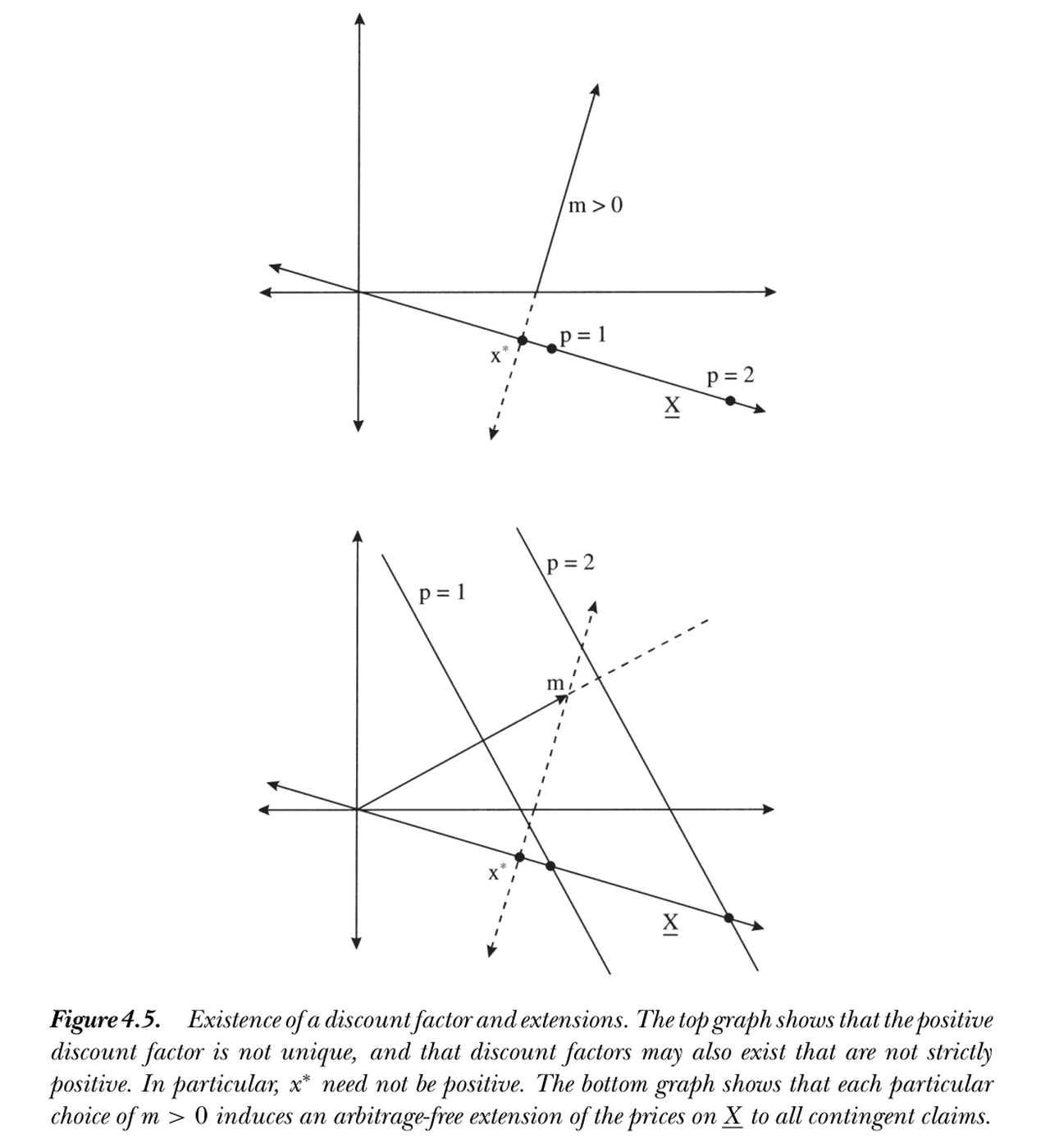
图 4.5　贴现因子的存在与扩张。上图：正贴现因子不唯一，且也存在不严格为正的贴现因子——$x^*$ 未必为正。下图：每一个 $m>0$ 都把 $\underline X$ 上的价格无套利地扩张到所有或有索取权。

Figure 4.5　Existence of a discount factor and extensions. Top: the positive discount factor is not unique, and discount factors that are not strictly positive exist too — $x^*$ need not be positive. Bottom: each choice of $m>0$ induces an arbitrage-free extension of the prices on $\underline X$ to all contingent claims.

4.3 另一种表达式与连续时间 / An Alternative Formula and Continuous Time

公式 (4.1) 用二阶矩 $\mathbb E(xx')$ 表示 $x^*$。换用均值与协方差 $\Sigma=\operatorname{cov}(x)$ 表示常更直观。令 $\mathbb E(x^*)$ 待定，可证

4.3 An Alternative Formula and Continuous Time

Formula (4.1) expresses $x^*$ via the second moment $\mathbb E(xx')$. It is often more intuitive to use means and the covariance matrix $\Sigma=\operatorname{cov}(x)$ instead. With $\mathbb E(x^*)$ to be determined, one can show

$$x^*=\mathbb E(x^*)+\bigl[p-\mathbb E(x^*)\,\mathbb E(x)\bigr]'\,\Sigma^{-1}\bigl(x-\mathbb E(x)\bigr),\qquad \Sigma=\operatorname{cov}(x).\tag{4.2}$$

(4.2) 把 $x^*$ 写成"常数 + 对去均值支付的回归"形式：贴现因子是支付的线性函数，回归系数由价格与协方差结构决定。对超额收益 $R^e$（价格为零）这一式简化为 Hansen and Jagannathan (1991) 用来构造贴现因子边界的形式——这是第 5 章 Hansen-Jagannathan 界的起点。

把这一构造推广到连续时间。设资产价格服从扩散过程，瞬时超额收益的漂移与扩散为 $\mu$ 与 $\sigma$，则贴现因子过程 $\Lambda$ 满足

(4.2) writes $x^*$ as "a constant plus a regression on demeaned payoffs": the discount factor is a linear function of the payoffs, with regression coefficients set by the prices and the covariance structure. For excess returns $R^e$ (zero price) this reduces to the form Hansen and Jagannathan (1991) use to build discount-factor bounds — the starting point for the Hansen-Jagannathan bounds of Ch 5.

This construction extends to continuous time. With asset prices following diffusions whose instantaneous excess returns have drift $\mu$ and diffusion $\sigma$, the discount-factor process $\Lambda$ satisfies

$$\frac{d\Lambda}{\Lambda}=-r^f\,dt-\bigl(\mu+D/p-r^f\bigr)'\,\Sigma^{-1}\sigma\,dz,\qquad \Sigma=\sigma\sigma'.\tag{4.3}$$

(4.3) 是 (4.2) 的连续时间对应：贴现因子的漂移给出无风险利率 $-r^f$，其扩散载荷由资产的瞬时超额收益（含红利率 $D/p$）经协方差 $\Sigma=\sigma\sigma'$ 调整后决定。$x^*$（以及 $\Lambda$）始终是落在可交易资产张成空间内的那个贴现因子。

(4.3) is the continuous-time counterpart of (4.2): the drift of the discount factor gives minus the risk-free rate $-r^f$, and its diffusion loadings are set by the assets' instantaneous excess returns (including the dividend yield $D/p$), adjusted through the covariance $\Sigma=\sigma\sigma'$. As before, $x^*$ (and $\Lambda$) is the discount factor lying inside the span of the tradeable assets.

小结 / Summary

本章的逻辑链非常干净：一价定律 $\Rightarrow$ 存在贴现因子 $x^*$（公式 (4.1)，但未必为正）；无套利 $\Rightarrow$ 存在正贴现因子 $m>0$（分离超平面，但不唯一）。$x^*=\operatorname{proj}(m\mid X)$ 是 $m$ 在支付空间上的投影。完全市场下 $m=x^*$ 唯一；不完全市场下，$m>0$ 的多样性恰对应给不可交易支付定价的自由度。这为后续 Hansen-Jagannathan 界、贝塔表示与因子模型铺平了道路。

Summary

The logic of this chapter is very clean: law of one price $\Rightarrow$ a discount factor $x^*$ exists (formula (4.1), but not necessarily positive); no-arbitrage $\Rightarrow$ a positive discount factor $m>0$ exists (separating hyperplane, but not unique). $x^*=\operatorname{proj}(m\mid X)$ is the projection of $m$ onto the payoff space. In a complete market $m=x^*$ is unique; in an incomplete market, the multiplicity of $m>0$ is exactly the freedom in how to price non-tradeable payoffs. This paves the way for the Hansen-Jagannathan bounds, beta representations, and factor models to come.

习题 / Problems

构造 $x^*$。 在两状态、两资产的例子中，由价格与支付用 (4.1) 显式算出 $x^*$，并验证它给两资产定出正确价格。
$x^*$ 可正可负。 举一个无套利但 $x^*$ 在某状态为负的例子，说明为何这不构成套利（提示：$x^*$ 本身未必是可交易支付里"非负且正概率为正"的那种）。
扩张的不唯一性。 在一个不完全市场里，画出两条不同的分离超平面，对应两个不同的 $m>0$，并说明它们给同一个可交易支付定出相同价格、却给某个不可交易支付定出不同价格。

Problems

Construct $x^*$. In a two-state, two-asset example, compute $x^*$ explicitly from prices and payoffs using (4.1), and verify it prices both assets correctly.
$x^*$ can be negative. Give an example with no arbitrage in which $x^*$ is negative in some state, and explain why this is not an arbitrage (hint: $x^*$ itself need not be one of the "non-negative, positive with positive probability" tradeable payoffs).
Non-uniqueness of the extension. In an incomplete market, draw two different separating hyperplanes corresponding to two different $m>0$, and show they assign the same price to a given tradeable payoff but different prices to some non-tradeable payoff.